Physics-Informed Neural Compression of High-Dimensional Plasma Data

TL;DR
Introduction
In the previous blogpost we introduced ![]() GyroSwin [1], a scalable 5D vision transformer able to reliably capture the full nonlinear dynamics of gyrokinetic plasma turbulence. In this post, we present a direction orthogonal to GyroSwin, tackling one of the main challenges that emerged from large-scale training on high-dimensional data: storage!
GyroSwin [1], a scalable 5D vision transformer able to reliably capture the full nonlinear dynamics of gyrokinetic plasma turbulence. In this post, we present a direction orthogonal to GyroSwin, tackling one of the main challenges that emerged from large-scale training on high-dimensional data: storage!
Indeed, to achieve its impressive results GyroSwin was trained on a “simple” dataset that consisted already of terabytes of plasma data. “Production” gyrokinetic simulations are orders of magnitude more expensive, both in terms of compute and storage required. From a machine learning perspective this would make it unfeasible to package a complete and diverse gyrokinetic dataset. On the plasma scientist side of the coin, entire simulations can never be stored at full resolution, and practictioners base their analysis on simpler integrated quantities, time traces and spectra.
Our attempt to ease both concerns is ![]() Physics-Inspired Neural Compression (PINC): we explore neural compression models (neural implicit fields [2] and Vector Quantized VAEs [3]) equipped with plasma-specific physics-informed losses [4], and achieve impressive results in terms of reconstruction quality, physics preservation and compression rates (with VQ-VAEs, up to 70,000x!).
Physics-Inspired Neural Compression (PINC): we explore neural compression models (neural implicit fields [2] and Vector Quantized VAEs [3]) equipped with plasma-specific physics-informed losses [4], and achieve impressive results in terms of reconstruction quality, physics preservation and compression rates (with VQ-VAEs, up to 70,000x!).
Our Approach
Evaluating Plasma Turbulence
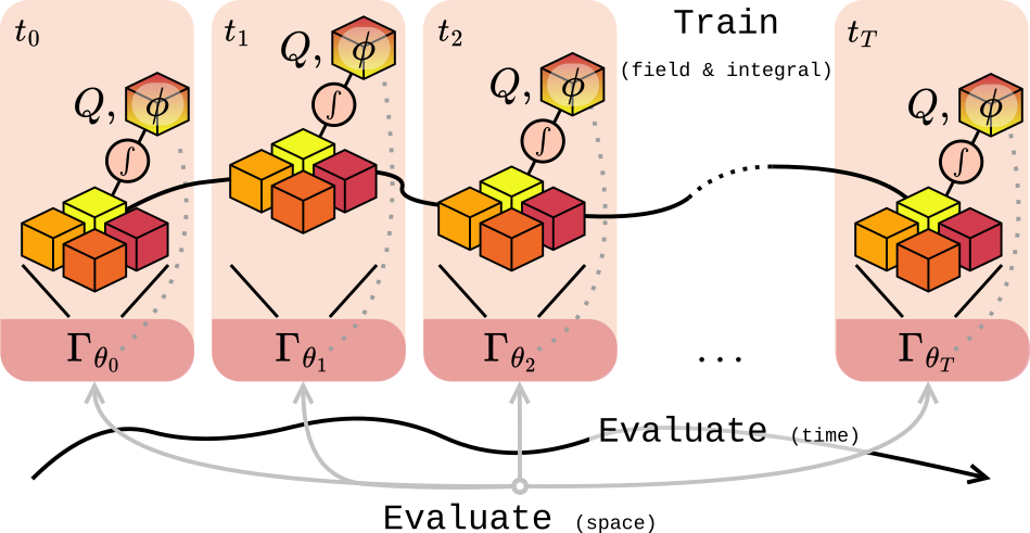
As described in the previous blogpost, the full representation of gyrokinetics is the 5D phase space distribution function \(\boldsymbol{f}\). To check whether compression keeps the physics intact, we look at both spatial and temporal measures of turbulence. Two core quantities come from integrating \(\boldsymbol{f}\) to obtain the electrostatic potential \(\boldsymbol{\phi}\) and heat flux \(Q\):
\[\boldsymbol{\phi} = \mathbf{A} \int \mathbf{J_{0}} \boldsymbol{f} \: \mathrm{d}v_{\parallel}\,\mathrm{d}\mu, \quad Q = \int \mathbf{B} \int \mathbf{v}^2 \boldsymbol{\phi} \boldsymbol{f} \: \mathrm{d}v_{\parallel}\mathrm{d}\mu \:\: \mathrm{d}x\,\mathrm{d}y\,\mathrm{d}s.\]Additionally, turbulence is interpreted by looking at how energy distributes across spatial modes, using wave-space diagnostics like \(k_y^{\text{spec}}\) and \(Q^{\text{spec}}\).
Neural Compression
We experiment with two dominant techniques:
- Autoencoders (AEs / VQ-VAEs): explicit compression through a latent bottleneck, parameters are shared across data.
- Neural Implicit Fields (NFs): store each snapshot as a tiny independent coordinate-based network, with compression happening implicitly in weight space.
Both optimize a complex MSE loss on the 5D distribution \(\boldsymbol{f}\)
\[\mathcal{L}_{\text{recon}} = \sum_{v_{\parallel}\mu s x y} \left[ \Re(\boldsymbol{f}_{\text{pred}} - \boldsymbol{f}_{\text{GT}})^2 + \Im(\boldsymbol{f}_{\text{pred}} - \boldsymbol{f}_{\text{GT}})^2 \right].\]Physics-Inspired Neural Compression
Plain reconstruction loss isn’t enough, and high reconstruction quality does not always reflect in the physical fidelity. PINC adds penalties on the ground truth physical quantities \(\boldsymbol{\phi}\) and \(Q\), as well as the diagnostic spectra \(k_y^{\text{spec}}\) and \(Q^{\text{spec}}\). Moreover, monotonicity of the energy cascade is enforced as a knowledge-driven physical constraint.
As a side note, while PINC-neural fields can be comfortably trained with off-the-shelf optimizers, the story is different for the more complex autoencoders. Instead, naively training them on all PINC losses often leads to severe instabilities and catastrophic forgetting. We solve this complication by pretraining the larger autoencoders on the distribution \(\boldsymbol{f}\), and subsequently using Explained Variance Adaptation [5] to finetune the model on the PINC losses.
Results
Quantitative
Learned compression shows strong performance on all metrics in our dataset. Neural fields and autoencoders with PINC losses considerably improve the conservation of physical quantities, compared to the unregularized counterparts. For neural fields, training on physics-informed losses degrades reconstruction quality slightly and introduces some temporal inconsistencies, and we speculate this is caused by conflict gradients.
| Method | CR | PSNR ↑ | EPE ↓ | L1(Q) ↓ | PSNR(\(\phi\)) ↑ | WD(\(k_y^{\text{spec}}\)) ↓ | WD(\(Q^{\text{spec}}\)) ↓ |
|---|---|---|---|---|---|---|---|
| ZFP | 901× | 28.97 ± 1.09 | 0.175 ± 0.07 | 107.48 ± 49.35 | −16.20 ± 7.09 | 0.020 ± 0.01 | 0.116 ± 0.20 |
| Wavelet | 936× | 33.07 ± 1.18 | 0.064 ± 0.03 | 107.74 ± 49.51 | −13.24 ± 9.20 | 0.020 ± 0.01 | 0.010 ± 0.00 |
| PCA | 1020× | 32.09 ± 0.98 | 0.123 ± 0.07 | 67.60 ± 36.08 | −10.22 ± 6.89 | 0.020 ± 0.01 | 0.011 ± 0.00 |
| JPEG2000 | 1000× | 34.33 ± 0.95 | 0.046 ± 0.02 | 103.91 ± 44.12 | −20.85 ± 6.50 | 0.020 ± 0.01 | 0.035 ± 0.03 |
| NF | 1167× | 36.91 ± 0.93 | 0.031 ± 0.02 | 61.50 ± 16.91 | 1.24 ± 5.99 | 0.017 ± 0.01 | 0.017 ± 0.00 |
| PINC-NF | 1167× | 35.76 ± 1.38 | 0.037 ± 0.02 | 2.18 ± 8.33 | 13.50 ± 4.44 | 0.006 ± 0.00 | 0.015 ± 0.00 |
| AE + EVA | 716× | 35.64 ± 2.03 | 0.063 ± 0.05 | 15.01 ± 16.42 | 6.72 ± 4.98 | 0.016 ± 0.01 | 0.012 ± 0.01 |
| VQ-VAE + EVA | 301× | 32.61 ± 1.58 | 0.095 ± 0.07 | 44.26 ± 40.97 | 7.66 ± 3.75 | 0.015 ± 0.01 | 0.013 ± 0.01 |
This table is obtained from the public 50GB dataset, and can be reproduced with the evaluation notebook 01_pinc_evaluation_hf.ipynb.
Qualitative
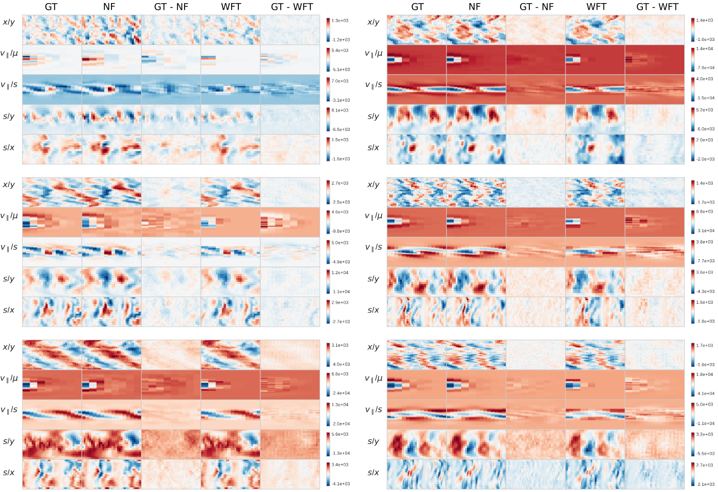
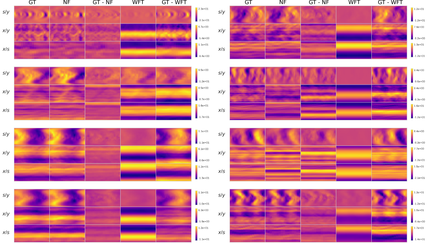
Figure 2: Reconstructions for the density (a) and electrostatic potential (b) for a few randomly picked snapshots across different trajectories.
These 2D projections of the 5D (left) and 3D (right) fields demonstrate the advantage of PINC neural fields in direct density reconstruction, and even more clear for integral fidelity for the electrostatic potential. This is reflected in the higher \(\boldsymbol{\phi}\) PSNR in Table 1.
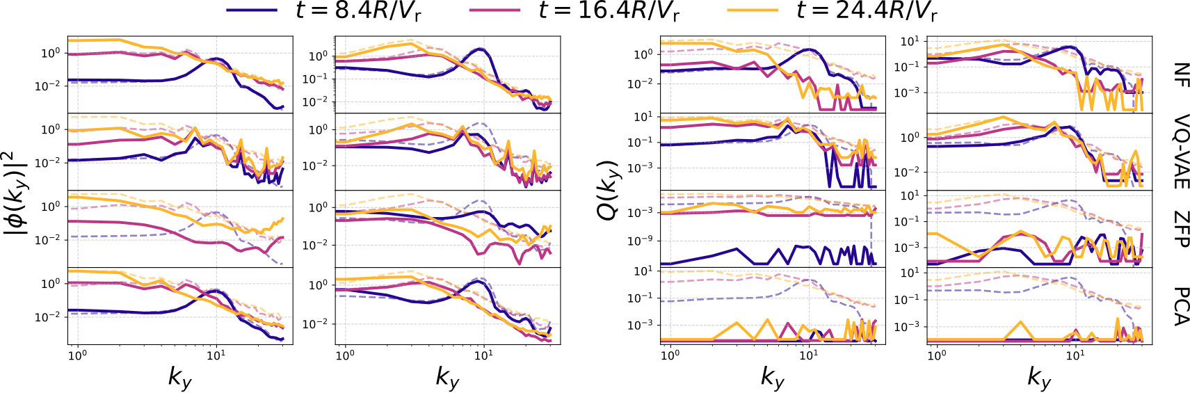
Figure 3 visualizes the bi-directional energy cascade phenomenon: as turbulence develops, energy is transferred from higher to lower modes and vice-versa. Columns are different trajectories, rows are compression methods, lines of varied colors are the \(k_y^{\text{spec}}\) and \(Q^{\text{spec}}\) at specific timesteps, and transparent dashed lines are respective ground truth.
While traditional compressoin techniques sometimes manage to visually capture \(k_y^{\text{spec}}\), they fail completely on \(Q^{\text{spec}}\). On the other hand, PINCs are somewhat less accurate on high frequencies, but generally capture low frequencies and magnitude pretty well.
Rate-Distortion scaling
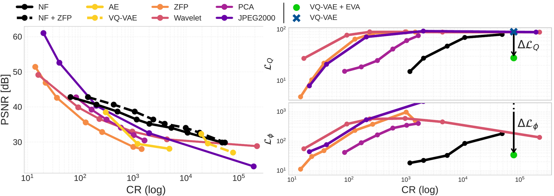
The left figure highlights an advantageous power-law scaling for the neural fields, against a super-exponential decay for traditional compression techniques. We also notice a “goldilocks compression rate” , between 200x and 10,000x where neural fields outperform traditional compression on direct reconstruction.
The right plot shows the improvement of PINC training in terms of the integral loss gap, reported for a single VQ-VAE (blue cross \(\to\) green dot, \(\Delta \mathcal{L}\) gap displayed with an arrow).
Conclusions and Future Work
PINC opens new possibilities for sharing, storing, and analyzing scientific datasets that were previously too large to handle. What’s next?
- Big small datasets. The initial concern that motivated this work is scaling GyroSwin to even larger data volumes, and especially higher fidelity data. With PINC, compressed representations can either be inflated in-transit, or directly serve as a dataset for “compressed” surrogate modeling. For instance, the VQ-VAE can be leveraged for latent diffusion, where turbulent solutions are generated starting from operational parameters.
- Integration into numerical codes and workflows. Integrating PINC in the plasma scientist workflow of GKW would enable cheap, staggered on-the-fly (in-situ) compression during the simulation, making it feasible to capture transient dynamics without writing massive data dumps to disk.
Resources
Citation
If you found our work useful, please consider citing it.
@misc{galletti2026physicsinformedneuralcompressionhighdimensional,
      title={Physics-Informed Neural Compression of High-Dimensional Plasma Data},
      author={Gianluca Galletti and Gerald Gutenbrunner and Sandeep S. Cranganore and William Hornsby and Lorenzo Zanisi and Naomi Carey and Stanislas Pamela and Johannes Brandstetter and Fabian Paischer},
      year={2026},
      eprint={2602.04758},
      archivePrefix={arXiv},
      primaryClass={physics.plasm-ph},
      url={https://arxiv.org/abs/2602.04758},
}
References
[1] Fabian Paischer, Gianluca Galletti, William Hornsby, Paul Setinek, Lorenzo Zanisi, Naomi Carey, Stanislas Pamela, and Johannes Brandstetter, “GyroSwin: 5D Surrogates for Gyrokinetic Plasma Turbulence Simulations” in Advances in Neural Information Processing Systems 38 (NeurIPS 2025) https://arxiv.org/abs/2510.07314
[2] Ben Mildenhall, Pratul P. Srinivasan, Matthew Tancik, Jonathan T. Barron, Ravi Ramamoorthi, and Ren Ng, “NeRF: Representing Scenes as Neural Radiance Fields for View Synthesis,” arXiv preprint arXiv:2003.08934, 2020. [Online]. Available: https://arxiv.org/abs/2003.08934
[3] Aaron van den Oord, Oriol Vinyals, and Koray Kavukcuoglu, “Neural Discrete Representation Learning,” arXiv preprint arXiv:1711.00937, 2018. [Online]. Available: https://arxiv.org/abs/1711.00937
[4] George E. Karniadakis, Ioannis G. Kevrekidis, Lu Lu, et al., “Physics-informed machine learning,” Nature Reviews Physics, vol. 3, pp. 422–440, 2021. [Online]. Available: https://doi.org/10.1038/s42254-021-00314-5
[5] Fabian Paischer, Lukas Hauzenberger, Thomas Schmied, Benedikt Alkin, Marc Peter Deisenroth, and Sepp Hochreiter, “Parameter Efficient Fine-tuning via Explained Variance Adaptation,” arXiv preprint arXiv:2410.07170, in Advances in Neural Information Processing Systems 38 (NeurIPS 2025) https://arxiv.org/abs/2410.07170
2025, Gianluca Galletti