GyroSwin: 5D Surrogates for Gyrokinetic Plasma Turbulence Simulations
TL;DR
Introduction
Nuclear Fusion is a promising contender for sustainable energy production. For humans, we can use the energy released by the reaction of fusing two hydrogen atoms (to form helium and a neutron, where most energy ends up) to power, for example, a turbine. In nature, fusion naturally occurs in stars, where the strong gravitational force produces massive pressures which overcome the repelling force between two hydrogen atoms (Coulomb barrier). The figure below shows the fusion reaction for hydrogen isotopes Deutereum and Tritium.
Since the gravitational force on planet Earth is insufficient to overcome this barrier, we require massive amounts of heat to increase the probability of atoms fusing. In reality, this means heating up a gas to hundreds of millions of degrees, which is also called a Plasma. At these conditions, hydrogen atoms split into ions and electrons. Due the amount of heat, the Plasma has to be confined within magnetic fields, as there is no material that could withstand such extreme temperatures.
To turn nuclar fusion into a viable energy source, Plasma needs to be confined over long periods of time. This is difficult, as it’s inherently unstable, and often tries to escape confinement. One contributor to this behavior is turbulence, which arises due to temperature gradients within the Plasma. Therefore it is essential to understand and model Plasma turbulence in modern reactors such as Tokamaks, in order to downstream design new reactors and confinement control systems. However, understanding and modelling Plasma turbulence is an incredibly hard problem, and practictioners must rely on expensive numerical simulations.
“Nuclear fusion is not rocket science, because it’s way harder.”
— William Hornsby
Because it promises sustainable, safe, and relatively affordable energy, nuclear fusion remains a key focus in the pursuit of securing our future energy supply.
The Problem
Understanding plasma turbulence is crucial for modelling plasma scenarios for confinement control and reactor design. Numerically, Plasma turbulence is governed by the nonlinear gyrokinetic equation, which evolves a 5D distribution function over time in phase space.
Let \(f = f(x, y, s, v_{\parallel}, \mu)\) where:
- \(x\), \(y\) are spatial coordinates along a toroidal C-section of a torus in real space.
- \(s\) is the toroidal coordinate along the field line, going around the torus.
- \(v_{\parallel}\) the parallel velocity component along the field lines.
- \(\mu\) is the magnetic angular moment, related to the gyral motion of particles.
The time-evolution of the perturbed distribution \(f\) , usually called \(\delta f\), is governed by the gyrokinetic equation [5, 6, 7], a reduced form of the Vlasov-Maxwell PDE system
\[\frac{\partial f}{\partial t} + (v_\parallel \mathbf{b} + \mathbf{v}_D) \cdot \nabla f -\frac{\mu B}{m} \frac{\mathbf{B} \cdot \nabla B}{B^2} \frac{\partial f}{\partial v_\parallel} + \mathbf{v}_\chi \cdot \nabla f = S\]Where:
- \(v_{\parallel} \mathbf{b}\) is the motion along magnetic field lines.
- \(\mathbf{b} = \mathbf{B} / B\) is the unit vector along the magnetic field \(\mathbf{B}\) with magnitude \(B\).
- \(\mathbf{v}_D\) is the magnetic drift due to gradients and curvature in \(\mathbf{B}\).
- \(\mathbf{v}_\chi\) describes nonlinear drifts arising from crossing electric and magnetic fields.
- \(S\) is the source term that represents collisions between particles.
The nonlinear term \(\mathbf{v}_\chi \cdot \nabla f\) describes turbulent advection, and the resulting nonlinear coupling constitutes the computationally most expensive term. For more details on gyrokinetics and the derivation of the equation, check “The non-linear gyro-kinetic flux tube code GKW” from Arthur Peeters et al. [5] and “Gyrokinetics” by Xavier Gerbet and Maxime Lesur [6].
This duality is related to the Fokker-Planck equation [9], which describes the evolution of probability densities under drift and diffusion. The Fokker-Planck equation is derived from an SDE, such as the Ornstein–Uhlenbeck process (as the forward Kolmogorov), and so it links the distribution-based and SDE-based descriptions.
Fully resolved gyrokinetics simulations are prohibitively expensive and often times practitioners need to rely on reduced order models, such as quasilinear models (for example QuaLiKiz [10]). QL models are fast but severely limited in generalization and accuracy, as they entirely neglect the nonlinear term \(\mathbf{v}_\chi \cdot \nabla f\). However, machine learning (neural) surrogate models have the potential to overcome this limitation if we develop methodologies that can cope with the complex nature of 5D data.
Our Approach
Our intuition is that modeling the entire 5D distribution function is vital to accurately model and comprehend turbulence in Plasmas. Therefore we require techniques that can process 5D data. The classic repertoire of an ML engineer comprises a variety of different techniques. Let’s break it down whether there are suitable to proccess 5D data.
- Convolutions? There is no out-of-the-box convolution kernel for >3D, so they need to be implemented either directly, recursively, or in a factorized manner. Regardless, convolutions become expensive and memory-intensive. [11]
- Transformers? ViTs can be applied to any number of dimension (provided proper patching / unpatching layers), but their quadratic scaling makes them unfeasible in our 5D setting due to quickly growing sequence lengths. [12, 13]
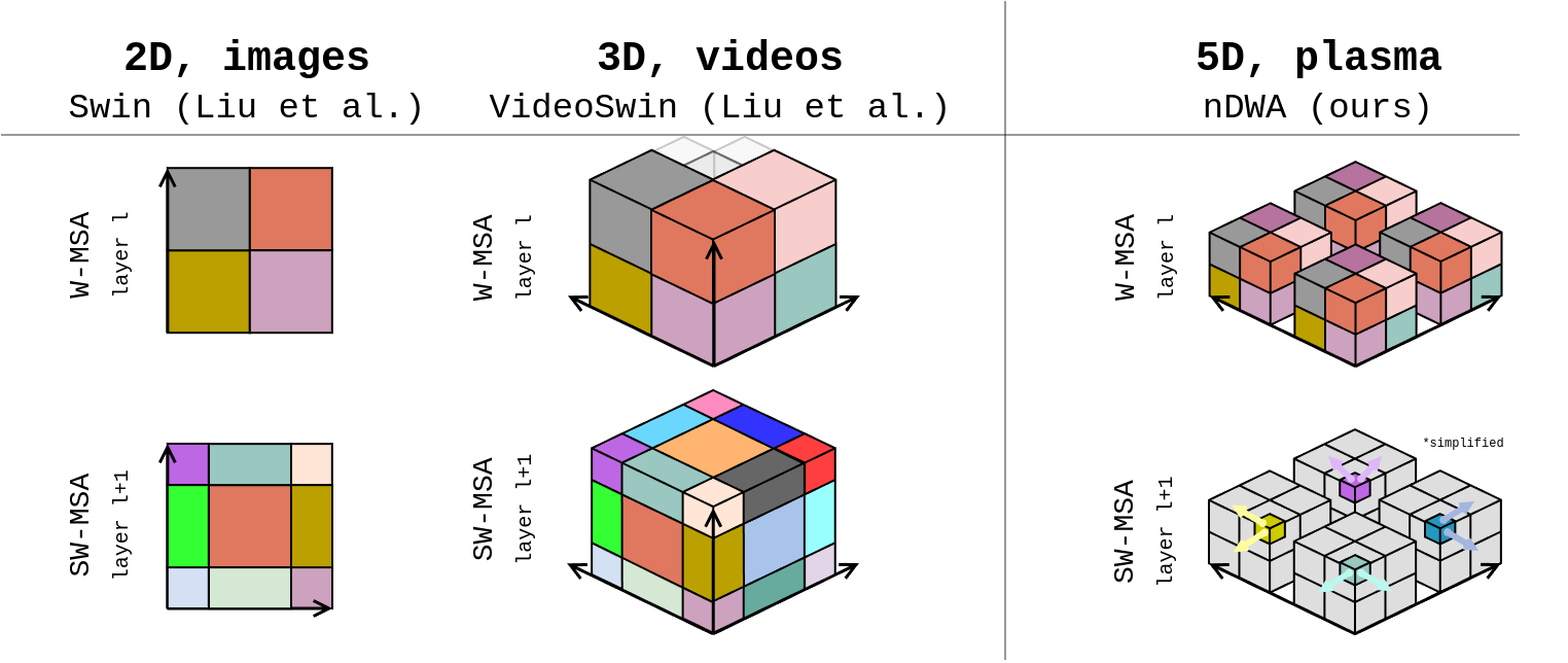
- Linear Attention? Vision Transformers with linear attention such as the Shifted Window Transformer (swin) [14] overcome quadratic scaling by performing attention locally in a simple way, making them an handy candidate for our case. However, to date, no implementation of swin Transformer exists that can process 5D data.
↪ There is no architecture out there that can natively handle 5D inputs. So, now what?
We generalize the local window attention mechanism used in Swin Transformers, together with patch merging and unpatching layers, to n-dimensional inputs. To this end, we generalize the (patch and window) partitioning strategy used in these layers to be able to process inputs of arbitrary dimensionalities. A standalone implementation of our n-dimensional swin layers can be found on github. The figure below provides an illustration on how we extend (shifted) window attention to n dimensions.
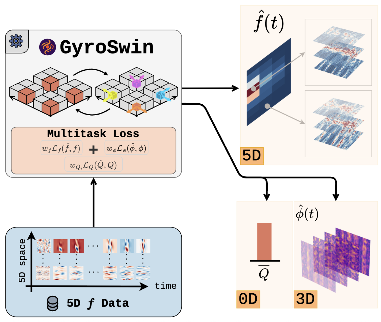
We propose Gyrokinetic Swin, ![]() GyroSwin, the first ever neural surrogate for nonlinear Gyrokinetic simulations. We start from the popular UNet architecture [15] and model the temporal evolution of the distribution function in an autoregressive manner. Furthermore, GyroSwin is a multitask model and not only predicts the evolution of the 5D distribution function, but also 3D potential fields and heat flux, which are usually obtained by performing complex integrals on the 5D fields. GyroSwin achieves this through three output branches at different dimensions whose latents communicate via cross attention.
GyroSwin, the first ever neural surrogate for nonlinear Gyrokinetic simulations. We start from the popular UNet architecture [15] and model the temporal evolution of the distribution function in an autoregressive manner. Furthermore, GyroSwin is a multitask model and not only predicts the evolution of the 5D distribution function, but also 3D potential fields and heat flux, which are usually obtained by performing complex integrals on the 5D fields. GyroSwin achieves this through three output branches at different dimensions whose latents communicate via cross attention.
Experiments
Data Generation
To explore how turbulence evolves under different plasma conditions, we ran a large series of nonlinear simulations using the GKW code. In each run, we varied the noise level of the initial conditions and four key operating parameters: the safety factor (\(q\)), magnetic shear (\(\hat{s}\)), ion temperature gradient (\(R/L_t\)), and density gradient (\(R/L_n\)).
Because these simulations are computationally expensive, we simplified the setup using the adiabatic electron approximation. This allowed us to focus on turbulence driven primarily by ion temperature gradients, while keeping a reasonably fine spatial resolution of (32 × 8 × 16 × 85 × 32).
In total, we generated 255 simulations. From these, we built two main training sets: a smaller one with 48 simulations for comparing baseline methods, and a larger one with 241 simulations for scaling studies. Altogether, this produced 44,585 training samples, including 8,880 from the smaller subset.
Baselines
The general landscape of surrogate models for gyrokinetics can be classified into tabular regressors, reduced-numerical models, and neural surrogates. Each of those have different characteristics and capabilities, as seen in the table below. For example, neural surrogates operating in 5D can model heat flux, can be used to compute diagnostics, model zonal flows, and turbulence itself. Reduced numerics can only be used for flux prediction and diagnostics. Finally, tabular regressors map operating parameters to heat flux.
| Method | Average Flux | Diagnostics | Zonal Flows | Turbulence |
|---|---|---|---|---|
| Tabular Regressors (e.g., GPR, MLP) | ✅ 1D → 0D | ❌ | ❌ | ❌ |
| SOTA Reduced Numerical Modelling (e.g., QL) | ✅ 3D → 0D | ✅ 3D → 1D | ❌ | ❌ |
| Neural Surrogates (e.g., GyroSwin) | ✅ 5D → 0D | ✅ 5D → 1D | ✅ 5D → 1D | ✅ 5D → 5D |
Evaluation
The key promise of our method is that it can step in where reduced numerical models fall short. Unlike QL approaches, which rely on simplified physics, our model is trained directly on the full 5D distribution function, capturing much richer dynamics, while remaining efficient and scalable.
To truly test whether our model delivers better performance than QL models, we conducted data collection in a regime dominated by strong ion temperature gradients. This ensures that the simulations reflect a high-turbulence environment, pushing both models to their limits.
Out of the 255 total simulations, we set aside 14 for evaluating how well the model generalizes. These are split into in-distribution (ID) and out-of-distribution (OOD) test cases.
For the ID set, we selected simulations that appear within the convex hull of the operating parameter space covered by training, but that the model hasn’t seen before. The OOD set is outside that convex region, forcing the model to make predictions in unfamiliar territory.
In total, we used six simulations for the ID evaluation and five for the OOD. The remaining three simulations served as a validation set during training. Importantly, none of these were ever part of the training data, ensuring that our evaluation truly reflects the model’s ability to generalize beyond what it has learned.
Results
For comparison to other surrogate approaches we use the smaller training set as training on the larger set is very expensive and, as we will show, most of the baselines do not scale too well.
5D\(\rightarrow\)5D Turbulence Modelling As a first result we quantify how well different methods capture turbulence and how stable they are during autoregressive rollouts in the table below. We quantified this stability using correlation time (CT), which measures how many consecutive snapshots the model can accurately predict while maintaining a certain level of Pearson correlation (denoted by \(\tau\)) with the true simulation data. The longer the correlation time, the better the model is at maintaining consistency over time. In the table below we report results for \(\tau=0.1\). When we compared different neural surrogate models, one result stood out clearly: our method was by far the most stable in autoregressive rollouts. Even more impressive, when we scaled up both the dataset size and the model itself, it achieved stable predictions for over 100 timesteps — and that held true even for OOD simulations that the model had never seen before.
5D\(\rightarrow\)0D Average flux prediction In this experiment, the goal was to predict the average heat flux (\(\bar{Q}\)) during the final phase of each simulation (over the last 80 timesteps) using 5D snapshots produced after an autoregressive rollout. On the smaller training set, our method clearly outperformed both the traditional quasilinear (QL) model and other 5D neural surrogates. Interestingly, many of the competing neural models tended to converge toward similar predicted values of heat flux. This happens because of error accumulation — as predictions become noisier over time, the computed average heat flux tends to rise artificially. In fact, if the predictions were completely random, we would see \(\bar{Q}\) values exceeding 1000, illustrating just how strongly error buildup can inflate the results.
What’s particularly exciting is that when we scale our method — training it on more data and using a larger model — the improvement is dramatic. The predictions become far more accurate, and the model achieves substantially lower error than any of the existing surrogate approaches.
| Method | Input | CT ID (\(\uparrow\)) | CT OOD (\(\uparrow\)) | \(\bar{Q}\) ID (\(\downarrow\)) | \(\bar{Q}\) OOD (\(\downarrow\)) |
|---|---|---|---|---|---|
| QL (Bourdelle et al., 2007) | 3D | n/a | n/a | 89.53 ± 11.76 | 95.22 ± 21.57 |
| Tabular regressors | |||||
| GPR (Hornsby, 2024) | 0D | n/a | n/a | 43.82 ± 10.84 | 59.28 ± 17.55 |
| MLP | 0D | n/a | n/a | 50.50 ± 10.79 | 61.98 ± 18.41 |
| Neural Surrogate Models (48 simulations) | |||||
| FNO (Li et al., 2021) | 3D | 9.33 ± 0.56 | 9.20 ± 0.58 | 119.88 ± 13.15 | 124.96 ± 23.27 |
| PointNet (Qi et al., 2016) | 5D | 7.33 ± 0.21 | 7.40 ± 0.24 | 119.93 ± 13.15 | 125.05 ± 23.29 |
| Transolver (Wu et al., 2024) | 5D | 9.83 ± 1.40 | 10.80 ± 1.46 | 119.93 ± 13.15 | 125.05 ± 23.28 |
| ViT (Dosovitskiy et al., 2021) | 5D | 16.83 ± 1.49 | 19.20 ± 1.36 | 119.63 ± 13.13 | 125.13 ± 23.29 |
| GyroSwin | 5D | 26.50 ± 3.55 | 28.60 ± 8.82 | 67.68 ± 10.28 | 70.48 ± 17.21 |
| Scaling GyroSwin to 241 simulations | |||||
| GyroSwin (small) | 5D | 98.00 ± 27.53 | 76.40 ± 17.60 | 23.72 ± 4.05 | 53.54 ± 18.10 |
| GyroSwin (medium) | 5D | 94.17 ± 21.96 | 91.20 ± 18.61 | 37.24 ± 9.60 | 44.17 ± 17.68 |
| GyroSwin (large) | 5D | 110.33 ± 19.74 | 111.80 ± 23.86 | 18.35 ± 1.56 | 26.43 ± 9.49 |
Scalability
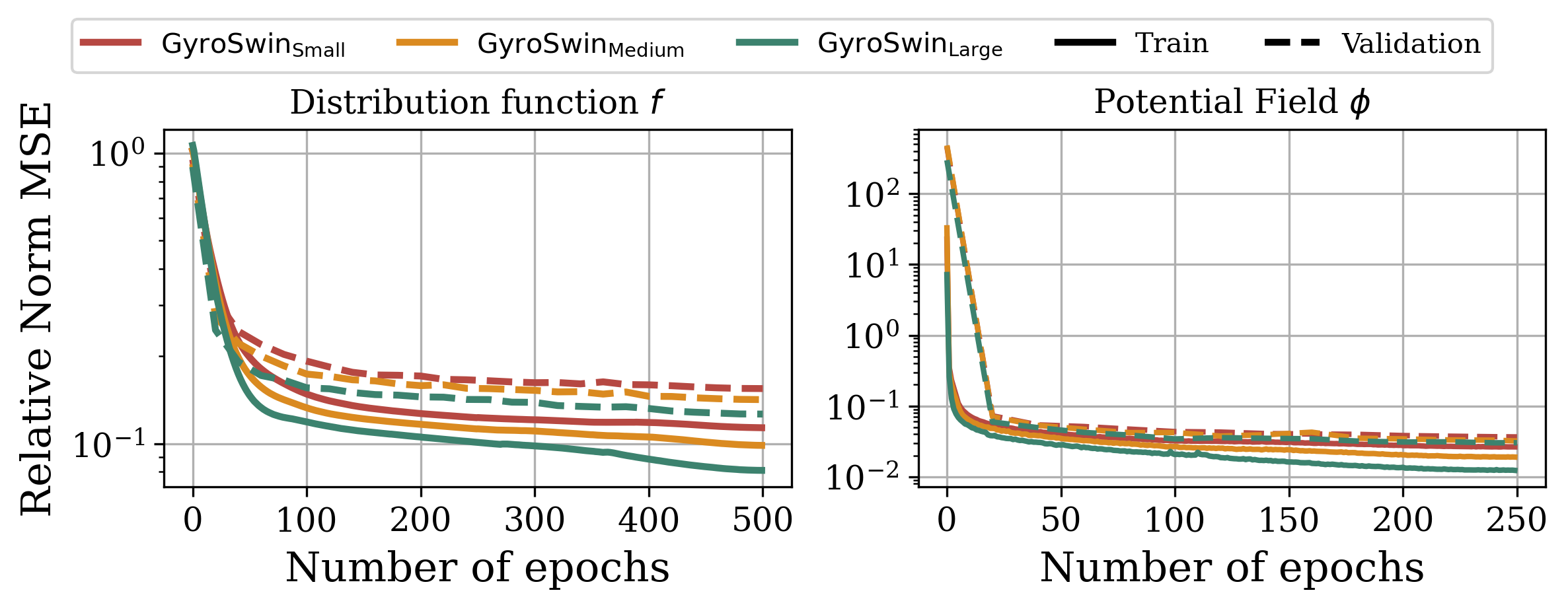
In integrated plasma simulations, turbulent heat fluxes must be repeatedly computed across thousands of runs, radial locations, and time intervals, underscoring the need for scalable surrogate architectures. The baselines we compared to in the table above lack this capability due to different reasons: (i) Convolution-based (CNN, FNO) require factorized implementations in 5D that are memory and time intensive, (ii) field-based methods (Transolver, PointNet) suffer from subsampling during training and chunked inference, (iii) vanilla ViTs suffer from quadratic complexity. Since GyroSwin is based on linear attention, we can scale it to train on 241 simulations which amounts to over 6TB of data. We observe intriguing scaling laws, indicated by a steady decrease in loss for increasing model sizes.
Does GyroSwin capture underlying physics?
Diagnostics are useful to assess whether a surrogate model accurately represents the underlying physics. One such diagnostic is the turbulence intensity spectrum \(W(k_y)\), which shows what modes in \(k_y\) contribute most to turbulence.
We visualize this spectrum for all neural surrogates and the QL model in the left figure below. We observe that while all neural surrogates decently reproduce the shape of the spectrum, they heavily underestimate the magnitude. Furthermore, GyroSwin matches shape and magnitude almost perfectly, except for a slight discrepancy for a few higher frequency components. We attribute this finding to the spectral bias of neural networks towards lower frequency (higher energy) modes [16]
Another intriguing nonlinear phenomena are zonal flows. They arise naturally with emerging turbulence in a plasma and regulate the system to reach a statistically steady state. They are only captured in the nonlinear term of gyrokinetics, therefore QL models cannot model them. However, they play a vital role in turbulence simulation as their amplitude determines the strength of emerging turbulence.
We can investigate whether GyroSwin is capable of capturing such zonal flows as they are represented as an isolated mode in the \(k_y\) dimension. The right figure below shows the profile, time-averaged for an OOD case, as well as GyroSwin’s prediction thereof. As we can see the zonal flow profile aligns very well with the ground-truth, indicating that GyroSwin indeed captures nonlinear physics.
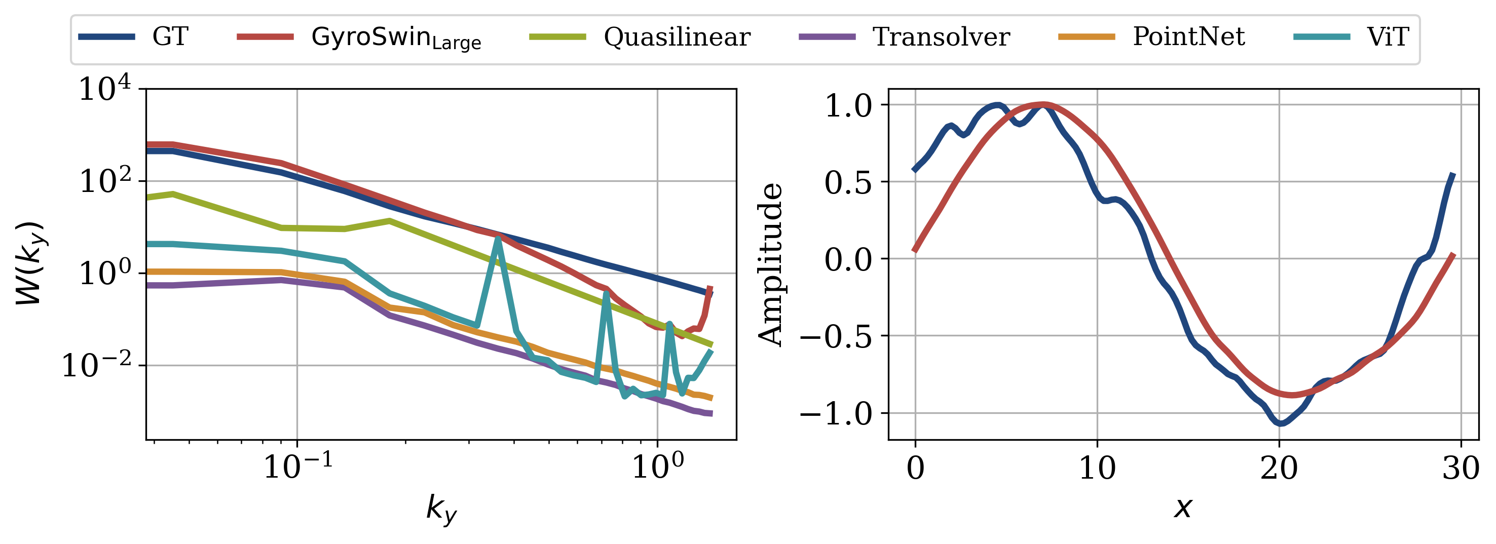
Figure 6: Left: Turbulence-intensity spectrum \(W(k_y)\) averaged over time and OOD simulations for different 5D neural surrogates. Competitors tend to underestimate while GyroSwin matches the spectrum well with a slight discrepancy on higher frequencies. Right: Time-averaged zonal flow profile for a slice along \(s\) across radial coordinates \(x\) for a selected OOD simulation. GyroSwin captures the zonal flow profile.
Wrapping up
GyroSwin outperforms reduced numerical approaches and other neural surrogates in modelling plasma turbulence. It accurately captures nonlinear phenomena and spectral quantities self-consistently, while offering a speedup of three orders of magnitude compared to the numerical solver GKW [7]. Furthermore, GyroSwin scales favorably to larger amounts of data and model sizes compared to competitors, which is imperative to truly advance surrogate modelling to higher fidelity plasma turbulence simulations. As a result, GyroSwin offers a fruitful alternative to reduced numerical models for efficient approximation of turbulent transport. Finally, plasma turbulence modelling is an incredibly hard problem, but we believe that Machine Learning will disrupt the landscape of plasma turbulence modelling in the future.
Resources
Citation
If you found our work useful, please consider citing it.
  @inproceedings{paischer2025gyroswin,
    author       = {Fabian Paischer and Gianluca Galletti
                    and William Hornsby and Paul Setinek
                    and Lorenzo Zanisi and Naomi Carey
                    and Stanislas Pamela and Johannes Brandstetter
                },
    booktitle    = {Advances in Neural Information Processing Systems 38: Annual Conference
                  on Neural Information Processing Systems 2025, NeurIPS 2025, San Diego,
                  CA, USA, December 02 - 07, 2025},
    year         = {2025}
  }
References
[1] Francis F. Chen, Introduction to Plasma Physics and Controlled Fusion, 3rd ed., Springer, 2016.
[2] Craig Freudenrich, “Physics of Nuclear Fusion Reactions,” HowStuffWorks, Aug. 4, 2015. [Online]. Available: http://science.howstuffworks.com/fusion-reactor1.html
[3] J. Wesson, Tokamaks, 4th ed., Oxford University Press, 2011.
[4] S. Atzeni and J. Meyer-ter-Vehn, The Physics of Inertial Fusion: Beam Plasma Interaction, Hydrodynamics, Hot Dense Matter, Oxford University Press, 2004.
[5] A. G. Peeters et al., The non-linear gyro-kinetic flux tube code GKW, Computer Physics Communications, 180(12), 2650–2672, 2009.
[6] E. A. Frieman and L. Chen, “Nonlinear gyrokinetic equations for low-frequency electromagnetic waves in general plasma equilibria,” Phys. Fluids, vol. 25, no. 3, pp. 502–508, Mar. 1982.
[7] X. Garbet and M. Lesur, Gyrokinetics, Lecture notes, France, Feb. 2023. [Online]. Available: https://hal.science/hal-03974985
[8] C. K. Birdsall and A. B. Langdon, Plasma Physics via Computer Simulation, Taylor & Francis, 2004.
[9] H. Risken, The Fokker-Planck Equation: Methods of Solution and Applications, 2nd ed., Springer, 1989.
[10] A. Casati, J. Citrin, C. Bourdelle, et al., “QuaLiKiz: A fast quasilinear gyrokinetic transport model,” Computer Physics Communications, vol. 254, p. 107295, 2020.
[11] Y. LeCun, Y. Bengio, and G. Hinton, “Deep learning,” Nature, vol. 521, pp. 436–444, 2015.
[12] A. Vaswani, N. Shazeer, N. Parmar, et al., “Attention Is All You Need,” in Advances in Neural Information Processing Systems (NeurIPS), 2017.
[13] A. Dosovitskiy, L. Beyer, A. Kolesnikov, et al., “An Image is Worth 16x16 Words: Transformers for Image Recognition at Scale,” in International Conference on Learning Representations (ICLR), 2021.
[14] Z. Liu, Y. Lin, Y. Cao, et al., “Swin Transformer: Hierarchical Vision Transformer using Shifted Windows,” in Proceedings of the IEEE/CVF International Conference on Computer Vision (ICCV), 2021, pp. 10012–10022.
[15] O. Ronneberger, P. Fischer, and T. Brox, “U-Net: Convolutional Networks for Biomedical Image Segmentation,” in Medical Image Computing and Computer-Assisted Intervention (MICCAI), 2015, pp. 234–241.
[16] Nasim Rahaman, Aristide Baratin, Devansh Arpit, Felix Draxler, Min Lin, Fred A. Hamprecht, Yoshua Bengio, and Aaron C. Courville. On the spectral bias of neural networks. Proceedings of the 36th International Conference on Machine Learning, ICML 2019, 9-15 June 2019, Long Beach, California, USA, volume 97 of Proceedings of Machine Learning Research, pp. 5301–5310. PMLR, 2019.
2025, Gianluca Galletti, Fabian Paischer