This blog post explains the paper Few-Shot Learning by Dimensionality Reduction in Gradient Space, which introduces SubGD, a novel few-shot learning algorithm (presented at CoLLAs 2022).
SubGD is a few-shot learning method that restricts fine-tuning to a low-dimensional parameter subspace. This reduces model complexity and increases sample efficiency. SubGD identifies the subspace through the most important update directions during fine-tuning on training tasks.
The interactive plot below illustrates how SubGD exploits important update directions. Due to the restriction to a subspace, SubGD approaches the minimum more directly.
The interactive plot shows a random loss surface over two network parameters \(x\) and \(y\). Our goal is to find the point in parameter space with minimal loss, which is marked by the red square. We start the optimization procedure from a random initialization point and compare the paths that different algorithms would take. The purple line shows the trajectory of standard gradient descent. It always takes steps in the direction of steepest descent. We simulate the stochasticity of SGD by adding a small fraction of noise to the standard gradient descent directions. The wiggly orange line shows the resulting trajectory. The noise resembles the gradient noise in training of neural networks that arises from random sampling of mini-batches. We show the trajectory of SubGD in dark blue. In this illustrative example, the subspace is spanned by the starting point and the true optimum. Of course, in real applications the subspace will have more than one dimension and the global optimum may not be located in it. Nevertheless, this example shows how a constrained subspace can lead to more efficient learning. As explained above, in every step we compute the gradient of the loss, project it to the subspace and perform the parameter update in this subspace. The figure suggests that if the subspace is suitable for our task (i.e., the test task in a few-shot setting), SubGD’s training trajectories are more robust to noisy gradients.
Subspace Gradient Descent
SubGD identifies the subspace directly from the training trajectories. These are the trajectories of SGD on the individual training tasks. Each trajectory is represented by the vector pointing from the starting point of training to the end point. From the resulting vectors we then calculate the auto-correlation matrix. The eigendecomposition of this matrix yields the \(r\) eigenvectors with the highest eigenvalues. In practice, you can think of this procedure as a PCA on the uncentered training trajectories.
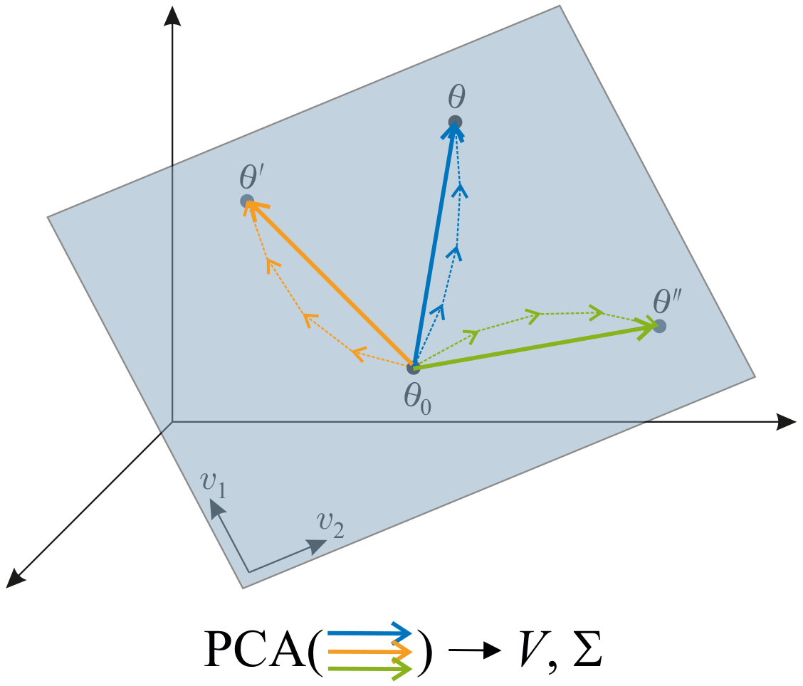
The most dominant eigenvectors (those with the highest eigenvalues) are the ones that were most important for fine-tuning; the subordinate eigenvectors were least important. Finally, we train on the test task, restricting gradient descent to the subspace of dominant eigenvectors, i.e., to the directions that are important to adapt to new tasks.
We could naively implement this restriction as projecting the gradient in the subspace of most important directions. However, we can do better than that and not just decide whether a direction is important, but also account for how important it is. This is exactly what the eigenvalues corresponding to the eigenvectors tell us! Instead of simply projecting on the subspace of important directions, we scale the learning rate for each direction individually with the eigenvalue. This way, we encourage parameter updates along the most important directions and discourage updates along other directions.
These ideas directly lead to the following update rule:

The update rule corresponds to the following operations on the gradient:
- \(\textcolor{#003f5c}{V^T} \in \mathbb{R}^{r \times n}\): transformation into the subspace
- \(\textcolor{#bc5090}{\Sigma} \in \mathbb{R}^{r \times r}\): scaling with diagonal matrix
- \(\textcolor{#003f5c}{V} \in \mathbb{R}^{n \times r}\): back-transformation into the full parameter space
Experimental Results
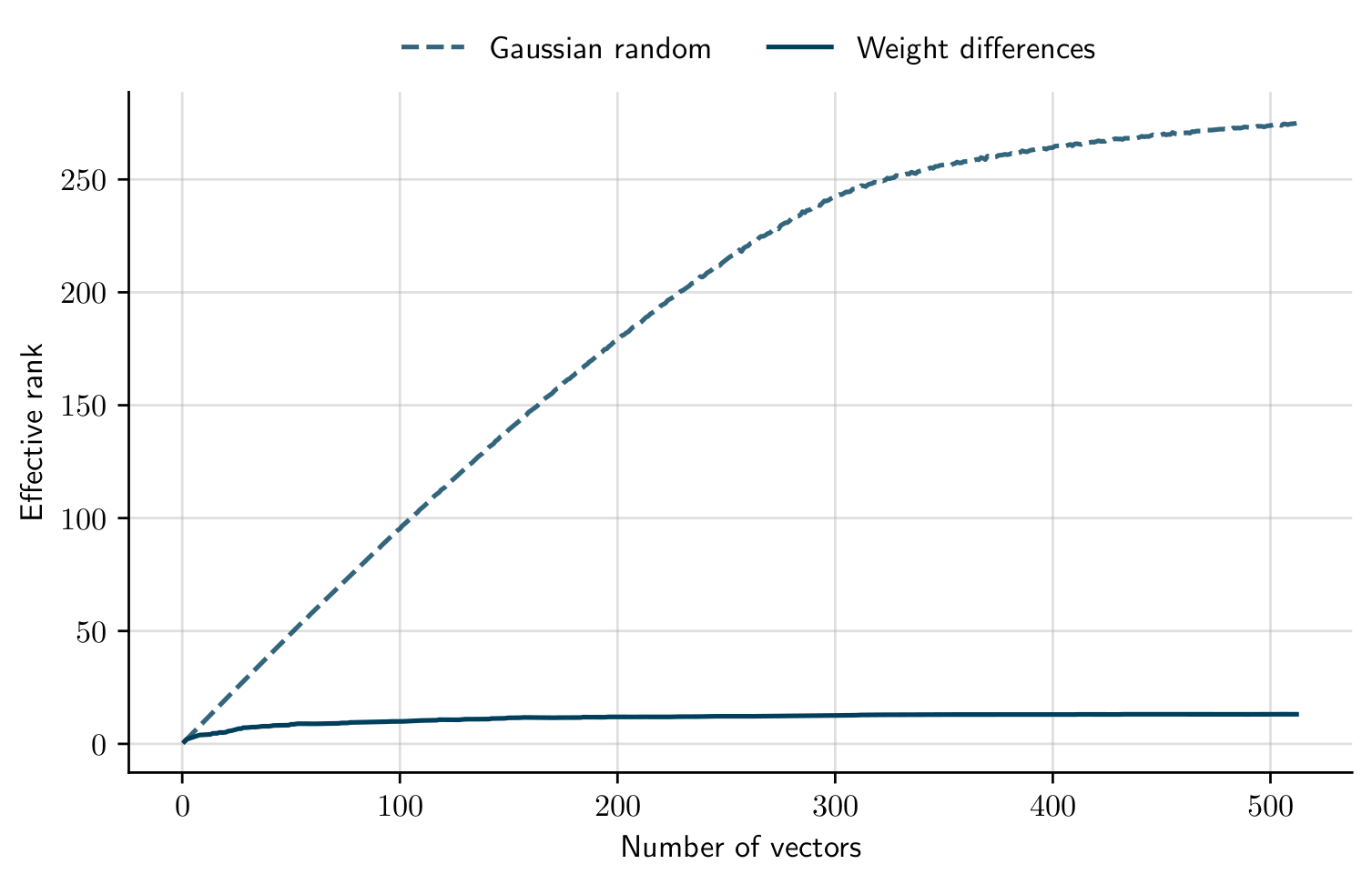
To be sure that SubGD works for a given few-shot learning setting, we must be able to identify a single low-dimensional subspace that allows learning in all tasks. We can measure the size of this subspace with the effective rank of the matrix of the training trajectories. The effective rank is a generalization of the normal matrix rank that does not only provide the number of subspace directions but also accounts for the variability along each direction. If the effective rank of our fine-tuning trajectories saturates as the number of tasks increases, we have found a subspace that SubGD can use to solve a new test task. In this case we would expect that applying SubGD should pay off. If, however, the effective rank increases with every new task, we can conclude that the tasks do not share a common subspace, and SubGD won’t work well.
Empirically, we find that the effective rank strongly depends on the few-shot learning setting. It turns out that SubGD is particularly well suited for dynamical systems — such as an electrical circuit (refer to our paper for more details on this setting). The effective rank curve flattens as we add more fine-tuning trajectories:
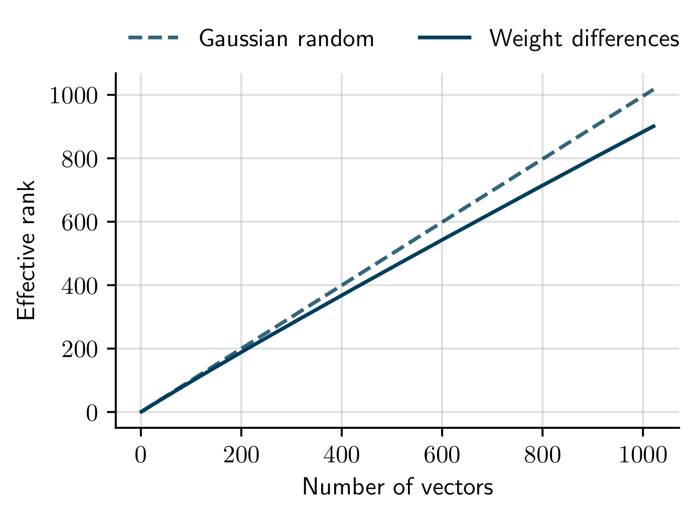
On the other hand, SubGD is not a good fit for many of the typical image-based few-shot learning tasks. For example, compare the above effective rank curve with that from miniImageNet tasks:
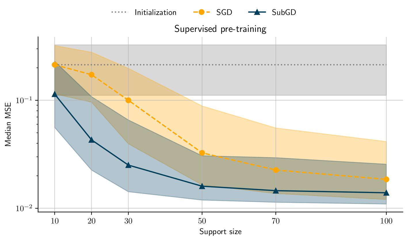
Still, in the cases where the effective ranks saturate, SubGD allows to adapt systems with high sample efficiency. The following plot compares the mean squared error (MSE) of normal fine-tuning against SubGD fine-tuning on tasks from the electrical circuit example as the amount of training samples (support size) increases:
Additional Material
Paper: https://arxiv.org/abs/2206.03483
Code on GitHub: https://github.com/ml-jku/subgd
Contact
gauch (at) ml.jku.at
This blog post was written by Martin Gauch, Maximilian Beck, Thomas Adler, Dmytro Kotsur, Stefan Fiel, Hamid Eghbal-zadeh, Johannes Brandstetter, Johannes Kofler, Markus Holzleitner, Werner Zellinger, Daniel Klotz, Sepp Hochreiter, and Sebastian Lehner.