This blog post explains HopCPT introduced in the paper “Conformal Prediction for Time Series with Modern Hopfield Networks which is accepted at Neurips2023.
HopCPT is an approach to generate prediction intervals for multivariate time series, given a point estimate from an arbitrary base prediction model. The learning-based Modern Hopfield architecture, in conjunction with the Conformal Prediction framework, exhibits distinctive properties that differentiate it from existing CP and non-CP approaches for estimating uncertainty in time series data:
- Locality/Conditionality: Unlike most Conformal Prediction Methods, HopCPT adapts its prediction interval to the local condition of the prediction. This leads to smaller prediction intervals and can improve the local coverage.
- Coverage Guarantees: HopCPT comes with approximation guarantees that the real prediction is included in the prediction interval. Due to its novel weighting technique, HopCPT can also preserve these guarantees in the challenging time series setting where the data is not i.i.d.
- Scaling: HopCPT is able to utilize the information across different time series of the same domain, is able to predict at different coverage levels without retraining, and is fast in inference.
HopCPT achieves a new state-of-the-art performance on 7 time series datasets from 4 different domains.
► Figure 1: Illustration of HopCPT
HopCPT find the relevant time steps of the past and retrieves its errors with a weighting. Then a weighted CP interval is build.HopCPT is built upon the framework of Conformal Prediction (CP). Conformal Prediction is used to generate reliable uncertainty estimates for an existing base predictor which only generated point predictions. Simply put, the idea of CP is to, first, apply a trained model to a calibration set and observe a so called non-conformity score of the prediction. In an regression setting the non-conformity score can be for example the absolute errors of the prediction. Then, given the set of errors, one calculates the $1-\alpha$ quantile, which directly provides the prediction interval boundaries by adding and subtracting the value to the point prediction. Given the data is exchangeable (if this concept is new to you, simply think of i.i.d.), it is guaranteed that for your test set, the prediction will be within the prediction interval with a probablity of $1-\alpha$.
However, there are two shortcomings of standard CP in its application to time series data: (1) The coverage guarantees of CP rely on the assumption that the data is exchangeable. However, time series data typically violates this assumption. (2) Standard CP only provided marginal coverage, meaning that given a calibration set, the prediction interval has a constant width. Since time series models often exhibit dynamical errors with local-specific behavior, this can result in unnecessarily large prediction intervals and potentially poor local coverage. An illustrative example for this can be seen in Figure 2 where the time series (prediction) inhibits two very different kind of error behavior. Here the standard CP intervals are unnecessary wide at large parts of the time series.
HopCPT overcomes both limitations by weighting the observed errors based on the similarity to the current prediction. This similarity measure is learned by a Modern Hopfield Network and incorporates the prediction value, the local features as well as temporal (distance) information. The quantile values for the prediction interval are then calculated based on this weighted set of errors, which are retrieved from the Hopfield memory. Figure 1 above illustrates this procedure. Intuitively spoken, HopCPT aims to find the time steps from the same error distribution as the current time step, so that the CP requirements are fulfilled.
For a more formal explanation check out the paper.
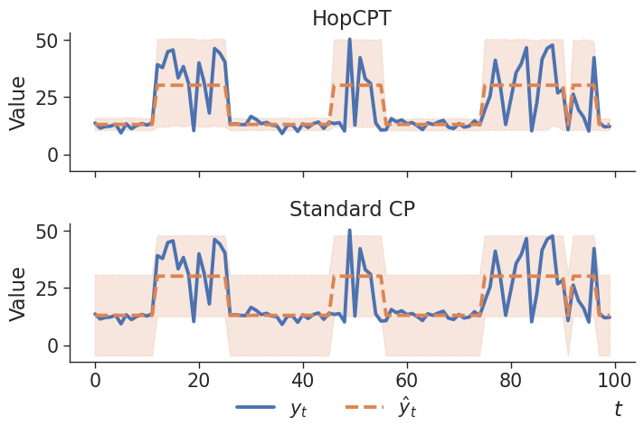
► Figure 2: HopCPT Vs. Standard CP
HopCPT is able to capture the different error distributions of the time series and adapts the prediction interval accordingly. Standard CP build only a marginal prediction interval which is very inefficent for the low error part of the time seriesExperimental Results
We evaluated HopCPT on 7 datasets from 4 different domains (solar energy, air quality, sap flow, streamflow) and compared it to multiple state-of-the-art conformal prediction methods for time series. The evaluation was conducted for different base prediction models. In addition, we also benchmarked HopCPT against state-of-the-art non-CP methods that are commonly used to generate uncertainty-aware prediction intervals.
The following two tables show results for miscoverage level $\alpha=0.1$, i.e. for the specification that 90% of the real values should be covered by the prediction interval. The tables present the results for a random forest and a LSTM base predictor. Results for other base predictor models and coverage levels, as well as a comparison to non-CP methods, can be found in the paper). Beside the $\Delta Cov$, which shows the deviation from the specified coverage level the tables show the PI-Width and Winkler Score. The PI-Width specifies the average width of the prediction interval - therefore a low PI-With is desirable because then the interval ist most informative. The Winkler score jointly considers the coverage criteria and the PI-Width and should be as low as possible. One can see that HopCPT outperform all competing methods by achieving the smallest PI-Width while preserving approximate coverage. This can be also easily seen by its low Winkler-Score compared to the other models.
Base Predictor: Random Forest
| Data | Metric | HopCPT | SPCI | EnbPi | NexCP | CopulaCPTS | CP/CF-RNN |
|---|---|---|---|---|---|---|---|
| Solar 3Y | $\Delta$ Cov | $0.029^{\pm 0.012}$ | $0.012^{\pm 0.000}$ | $-0.031$ | $-0.002$ | $0.005$ | $0.004$ |
| PI-Width | $\textbf{39.0}^{\pm 6.2}$ | $103.1^{\pm 0.1}$ | $131.1$ | $166.6$ | $174.9$ | $174.6$ | |
| Winkler | $\textbf{0.73}^{\pm 0.20}$ | $1.74^{\pm 0.00}$ | $2.47$ | $2.53$ | $2.75$ | $2.76$ | |
| Solar 1Y | $\Delta$ Cov | $0.047^{\pm 0.004}$ | $0.045^{\pm 0.000}$ | $-0.018$ | $0.002$ | $0.056$ | $0.063$ |
| PI-Width | $\textbf{28.6}^{\pm 1.0}$ | $97.1^{\pm 0.2}$ | $98.8$ | $127.8$ | $182.4$ | $204.9$ | |
| Winkler | $\textbf{0.40}^{\pm 0.04}$ | $1.26^{\pm 0.00}$ | $1.65$ | $1.84$ | $2.10$ | $2.30$ | |
| Solar Small | $\Delta$ Cov | $0.008^{\pm 0.006}$ | $-0.064^{\pm 0.002}$ | $-0.022$ | $-0.021$ | $-0.027$ | $-0.025$ |
| PI-Width | $\textbf{38.4}^{\pm 3.4}$ | $38.8^{\pm 0.3}$ | $86.0$ | $122.9$ | $110.4$ | $111.4$ | |
| Winkler | $\textbf{1.09}^{\pm 0.08}$ | $1.82^{\pm 0.01}$ | $2.54$ | $3.28$ | $3.47$ | $3.48$ | |
| Air 10 PM | $\Delta$ Cov | $0.028^{\pm 0.019}$ | $0.008^{\pm 0.000}$ | $-0.066$ | $-0.004$ | $-0.019$ | $-0.033$ |
| PI-Width | $\textbf{93.9}^{\pm 11.1}$ | $118.5^{\pm 0.1}$ | $202.8$ | $263.5$ | $243.1$ | $229.8$ | |
| Winkler | $\textbf{1.50}^{\pm 0.09}$ | $2.23^{\pm 0.00}$ | $4.16$ | $4.03$ | $4.94$ | $4.98$ | |
| Air 25 PM | $\Delta$ Cov | $-0.024^{\pm 0.017}$ | $-0.009^{\pm 0.000}$ | $-0.079$ | $-0.007$ | $-0.025$ | $-0.042$ |
| PI-Width | $\textbf{48.1}^{\pm 5.6}$ | $81.5^{\pm 0.0}$ | $177.3$ | $235.6$ | $212.6$ | $203.5$ | |
| Winkler | $\textbf{1.12}^{\pm 0.05}$ | $2.02^{\pm 0.00}$ | $4.31$ | $4.05$ | $4.94$ | $4.98$ | |
| Sap flow | $\Delta$ Cov | $0.009^{\pm 0.019}$ | $0.007^{\pm 0.000}$ | $-0.042$ | $0.000$ | $0.014$ | $0.005$ |
| PI-Width | $\textbf{1078.7}^{\pm 73.7}$ | $1741.8^{\pm 2.4}$ | $3671.6$ | $6137.1$ | $7131.1$ | $7201.5$ | |
| Winkler | $\textbf{0.30}^{\pm 0.01}$ | $0.59^{\pm 0.00}$ | $1.24$ | $1.56$ | $1.76$ | $1.80$ |
Base Predictor: LSTM
| Data | Metric | HopCPT | SPCI | EnbPi | NexCP | CopulaCPTS | CP/CF-RNN |
|---|---|---|---|---|---|---|---|
| Solar 3Y | $\Delta$ Cov | $0.001^{\pm 0.006}$ | $0.014^{\pm 0.000}$ | $-0.018$ | $-0.001$ | $0.007$ | $0.007$ |
| PI-Width | $\textbf{17.9}^{\pm 0.6}$ | $27.8^{\pm 0.0}$ | $24.6$ | $28.2$ | $31.9$ | $33.0$ | |
| Winkler | $\textbf{0.30}^{\pm 0.01}$ | $0.62^{\pm 0.00}$ | $0.64$ | $0.63$ | $0.68$ | $0.70$ | |
| Solar 1Y | $\Delta$ Cov | $0.028^{\pm 0.010}$ | $0.018^{\pm 0.000}$ | $-0.018$ | $-0.001$ | $0.018$ | $0.025$ |
| PI-Width | $\textbf{16.0}^{\pm 0.6}$ | $22.5^{\pm 0.0}$ | $17.4$ | $19.5$ | $23.1$ | $25.0$ | |
| Winkler | $\textbf{0.22}^{\pm 0.01}$ | $0.41^{\pm 0.00}$ | $0.42$ | $0.41$ | $0.43$ | $0.43$ | |
| Streamflow | $\Delta$ Cov | $0.001^{\pm 0.041}$ | $0.027^{\pm 0.000}$ | $-0.054$ | $-0.000$ | $0.005$ | $0.009$ |
| PI-Width | $\textbf{1.39}^{\pm 0.17}$ | $1.58^{\pm 0.00}$ | $1.55$ | $1.94$ | $1.99$ | $2.08$ | |
| Winkler | $\textbf{0.79}^{\pm 0.03}$ | $0.91^{\pm 0.00}$ | $1.27$ | $1.21$ | $1.28$ | $1.29$ | |
| Air 10 PM | $\Delta$ Cov | $-0.002^{\pm 0.005}$ | $0.010^{\pm 0.000}$ | $-0.025$ | $-0.002$ | $0.001$ | $0.004$ |
| PI-Width | $62.7^{\pm 1.5}$ | $62.2^{\pm 0.0}$ | $\textbf{58.1}$ | $62.4$ | $61.8$ | $63.0$ | |
| Winkler | $1.33^{\pm 0.01}$ | $\textbf{1.21}^{\pm 0.00}$ | $1.32$ | $1.29$ | $1.34$ | $1.34$ | |
| Air 25 PM | $\Delta$ Cov | $0.007^{\pm 0.008}$ | $-0.017^{\pm 0.000}$ | $-0.028$ | $-0.003$ | $-0.019$ | $-0.025$ |
| PI-Width | $40.7^{\pm 4.3}$ | $\textbf{32.4}^{\pm 0.0}$ | $35.9$ | $38.6$ | $34.0$ | $32.8$ | |
| Winkler | $\textbf{0.88}^{\pm 0.05}$ | $0.93^{\pm 0.00}$ | $0.97$ | $0.94$ | $0.99$ | $0.99$ | |
| Sap flow | $\Delta$ Cov | $0.004^{\pm 0.004}$ | $0.004^{\pm 0.000}$ | $-0.019$ | $-0.000$ | $-0.022$ | $-0.042$ |
| PI-Width | $\textbf{594.3}^{\pm 7.7}$ | $628.2^{\pm 0.9}$ | $768.0$ | $990.0$ | $903.9$ | $817.2$ | |
| Winkler | $\textbf{0.19}^{\pm 0.01}$ | $0.24^{\pm 0.00}$ | $0.28$ | $0.32$ | $0.35$ | $0.36$ |
►Table Information
Bold numbers correspond to the best result for the respective metric in the experiment (PI-Width and Winkler score). The error term represents the standard deviation over repeated runs with different seeds (results without an error term are from deterministic models)Check the paper for more detailed explanation about the overall experiment, data sets, compared models, hyperparameter tuning and other details. There you can also find additional evaluations, also to non-CP methods.
You can find an extensive set of additional experiments in the paper
Additional Material
Paper: Conformal Prediction for Time Series with Modern Hopfield Networks
Modern Hopfield Material: Blog: Hopfield Networks is All You Need
GitHub repository: hopfield-layers
This blogpost was written by Andreas Auer, Martin Gauch and Daniel Klotz
If there are any questions, feel free to contact us: auer[at]ml.jku.at